Author: Thomas Severin
Date: 15.Feb.2020
In this part I want to tell something about SciPy. It is an extension for Numpy.
SciPy contains modules for optimization, linear algebra, integration, interpolation, special functions, FFT, signal and image processing, ODE solvers and others.
Here I want to show you an example with B-splines. It is a subfield of numerical analysis. It has a wide range of applications like in the computer science subfields computer-aided design and computer graphics. It is also used for motion planning of robots and other mechanic structures.
B-splines were investigated in the beginning of the last century by Nikolai Lobachevsky. In the mathematics a spline is a smooth polynomial function that is piecewise-defined, and possesses a high degree of smoothness at the places where the polynomial pieces connect (which are called knots).
.
B-splines can be evaluated in a numerically stable way by the de Boor algorithm . I don't want to treat you here with this stuff of mathematical derivations. If you are more interested in this, you can read detailed information about computed geometry here here . The details and the derivation are also for me not of interest yet.
In SciPy is a function implemented to solve this stuff for you.
import matplotlib.pyplot as pp
import numpy as np
from scipy.interpolate import splprep, splev
Px = [1.0,2.0,3.0,4.0,5.0,6.0,32.0,8.0,9.0]
Py = [5.0,2.0,3.0,9.0,5.0,25.0,7.0,8.0,20.0]
#generating of the b-spline
tckp,u = splprep([Px,Py],s=3,k=2,nest=-1)
# evaluating (x-y-representation) of the b-spline
Pxnew,Pynew = splev(np.linspace(0,1,200),tckp)
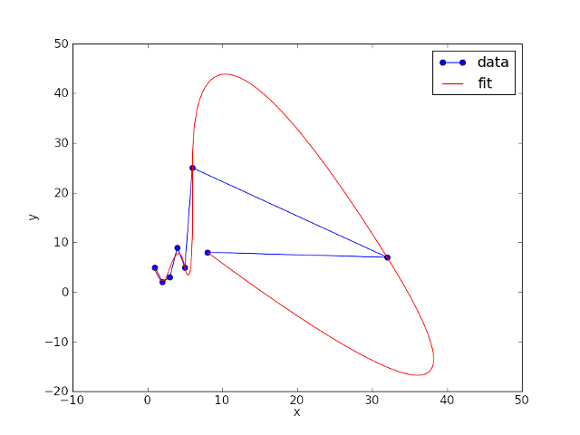
data,=pp.plot(Px,Py,'bo-',label='data')
fit,=pp.plot(Pxnew,Pynew,'r-',label='fit')
pp.legend()
pp.xlabel('x')
pp.ylabel('y')
pp.savefig('splprep.png')
pp.figure()
In line 1 is imported the package to plot the spline curve. In line 2 is imported the Numpy package for some array
functions and in scipy.interpolate are the necessary b-spline packages. In line 7 the splprep function finds the
B-spline representation of a curve. The factor k is the degree of the spline, while s is a smoothing condition which
is here of lower importance then the k factor. The tckp return value is a sequence of length 3 returned by splrep which
contains the knots, coefficients, and degree of the B-spline.
In line 9 the splev function is evaluating the B-spline. The linspace function, which is given as an argument,
creates an 1-diminsional array with 200 values between 0 and 1. It is the given resolution for the created B-spline curve.
This is one reason why the smoothness value s is of lower interest in this example.
The last lines are for plotting and legend configuration of the plot. The first plot command draws the points, the second command draws the B-spline.
This is a link to the scipy api.
Here is the result of this algorithm:
Here you can find some interpolation examples with scipy. Bye!